Combined Scale Out Networking Guide

The objectives for the network scheme for X200 are:

• Remove the limitation of 27 racks in a single deployment

• Easy scaleout with X100.

• Simplify configuration and ease requirements (routes / VLANs) for customer-supplied switches in large deployments, such as leaf-spine and Clos fabrics for very large scale-out and interconnection for 3 GEO (3GEO is not yet detailed in this guide).

• Be applicable and adaptable to many customer configurations

To make these objectives work, there were some decisions made to keep things scaleable and maintainable.

As a rule of thumb, X200 performance scales to 2GB/s PUT and 2.83GB/s per node for GET.

nodes per column	PUT performance (total)	GET performance (total)
6	12 GB/s	17 GB/s
12	24 GB/s	34 GB/s
18	36 GB/s	51 GB/s
24	48 GB/s	68 GB/s
30	60 GB/s	85 GB/s
36	72 GB/s	102 GB/s

The maximum network throughput per node is thus about 24GBit/s and with 2x25 Gbit/s per node available for the Public Network (customer-facing) and 2x25 Gbit/s per node for the Private Network (only erasure encoded data), a single-cluster ActiveScale X200 deployment (without JBOD) is not bottlecked by the network (if both ToR switches are up). [JBOD performance results pending]

The ActiveScale ToR switches for X200 (SMC) have 48 25GbE ports and 6 100GbE ports with support for layer 3 routing. 1 of the 48 25GbE ports on ToR 1 is used for the IPMI network. 36 can be used for ActiveScale nodes, and 11 25GbE are left, for instance for connecting to ActiveScale Cold Storage or to more switches for scaling out. A single column limit to 36 nodes is assumed in the design. The proposed IP network addressing would allow up to 48 node columns without modification (except the installer IP would need to be changed), but this is already tricky to achieve on a single switch.

The 2nd Gen Activescale will preferably use the following IP addressing scheme within the 172.20.0.0/14 address block. Each GEO x uses addresses in a 172.2x.0.0/16 range, and single GEO is in the 172.20.0.0/16 range. Separating single and 3GEO allows easy transition from single GEO to 3GEO.

• All Private Networks 1 (over ToR 1) are in the 172.2x.0.0/17 range

• All Private Networks 2 (over ToR 2) are in the 172.2x.128.0/17 range

Each column has two /24 subnets for the private networks: 172.2x.c.0/24 and 172.2x.(128+c).0/24, and each column has its own VLAN. While it is possible to put multiple columns in a single /24, putting each column on its own VLAN and IP subnet has many advantages: easier installation, full traffic isolation, no possible conflicting VLANs, no issues running applications that require broadcast, such as DHCP…

This addressing scheme allows to scale out (adding a new column to an existing deployment) to 128 columns per GEO.

This is not a hard limit (we can still add racks, starting over in 172.24.0.0/14 and 172.28.0.0/14 address block, etc), but this will suffice for the foreseeable future. In the odd event that these addresses conflict with the customer internal LAN network, it is recommended to adopt the numbering in one of the following blocks to resolve the conflict: 10.20.0.0/14, 10.120.0.0/14, 10.220.0.0/14

IP addresses in a column are assigned as follows:

1GEO	Private Network 1		Private Network 2
Scale out column	VLAN	IP subnet	VLAN	IP subnet
0 (base column)	1000	172.20.0.0/24	1128	172.20.128.0/24
1	1001	172.20.1.0/24	1129	172.20.129.0/24
2	1002	172.20.2.0/24	1130	172.20.130.0/24
…
127	1127	172.20.127.0/24	1255	172.20.255.0/24
3GEO	Private Networks 1		Private Networks 2
Scale out column	VLAN	IP subnets	VLANs	IP subnets
0 (base column)	1000 2000 3000	172.21.0.0/24 172.22.0.0/24 172.23.0.0/24	1128 2128 3128	172.21.128.0/24 172.22.128.0/24 172.23.128.0/24
1	1001 2001 3001	172.21.1.0/24 172.22.1.0/24 172.23.1.0/24	1129 2129 3129	172.21.129.0/24 172.22.129.0/24 172.23.129.0/24
2	1002 2002 3002	172.21.2.0/24 172.22.2.0/24 172.23.2.0/24	1130 2130 3130	172.21.130.0/24 172.22.130.0/24 172.23.130.0/24
127	1127 2127 3127	172.21.127.0/24 172.22.127.0/24 172.23.127.0/24	1255 2255 3255	172.21.255.0/24 172.22.255.0/24 172.23.255.0/24

IP Address Range in Subnet	Private Network 1	Private Network 2
001 - 036	AS node 1 - 36	AS node 1 - 36
101 - 136	IPMI interfaces AS node 1 - 36	-
151 - 174	PDU 1 - 24 (up to 4 / rack)	-
181 - 186	IPMI switches (1 / rack)	-
200	ToR Switch 1	ToR Switch 2
201 - 236	IPMI interfaces JBOD 1 - 18	-
240	Recommended IP for installer / VM during installation process	-

VLANs are numbered by GEO, starting at 1000, 2000, 3000, by column number for the Private Networks 1.

VLANs are numbered by GEO, starting at 1128, 2128, 3128, by column number for the Private Networks 2. So, when scaling out a deployment, the 25th scale out column in a 3-GEO would be on VLANs [1025, 1153] in GEO 1, [2025, 2153] in GEO2 and [3025, 3153] in GEO3. VLANs for a single GEO also start at 1000 (VLAN 0 is reserved). Should capability come for upgrading 1GEO to 3GEO, the GEOs 2 and 3 can be the same addresses and VLANs as in a “regular” 3GEO).

• The Private Network 1 ToR Switch is on address 200 within the Private network 1

• The Private Network 2 ToR Switch is on address 200 within the Private network 2

Routes for X200 scaleout can be predefined on each column c using only 2 entries:

172.2y.0.0/17 via 172.2x.c.200          for Private Network 1 172.2y.128.0/17 via 172.2x.(128+c).200  for Private Network 2

This allows a simple mapping between IP subnet and VLAN IDs to keep things manageable.
For instance, IP address 172.22.12.35 means the following:

• It’s in GEO 2 of a 3 GEO system (172.22.12.35)

• It’s on Private Network 1, (12 < 128) and VLAN 2012 (172.22.12.35)

• It’s the 12th column in this deployment (172.22.12.35)

• And the 35th node in the column (172.22.12.35)

• The IPMI address for the node is 172.22.12.135

• The IPMI addresses for the JBOD attached to the node are 172.22.12.235 and 172.22.12.236

• The ToR 1 switch can be reached on 172.22.12.200

• The ToR 2 switch can be reached on 172.22.140.200

The recommended IPMI network uses one IPMI switch per datacenter rack. The nodes and JBODs are connected via RJ45 to the IPMI switch in the same rack, IPMI switches are connected over SFP+ between racks. The IPMI switch in the base rack is connected to the ToR 1 in the same rack. The installer / VM can be connected to the IPMI network for installing ActiveScale. The IPMI switch allows connecting 5 JBOD + 5 twins and 4 PDUs in the same rack to be connected to its 24 RJ45 ports. For small deployments, the IPMI switch can be omitted and IPMI can be connected over RJ45-SPF convertors to ToR1, if the customer requests/insists.

ActiveScale X200 Racked 18 Twin Plus JBOD

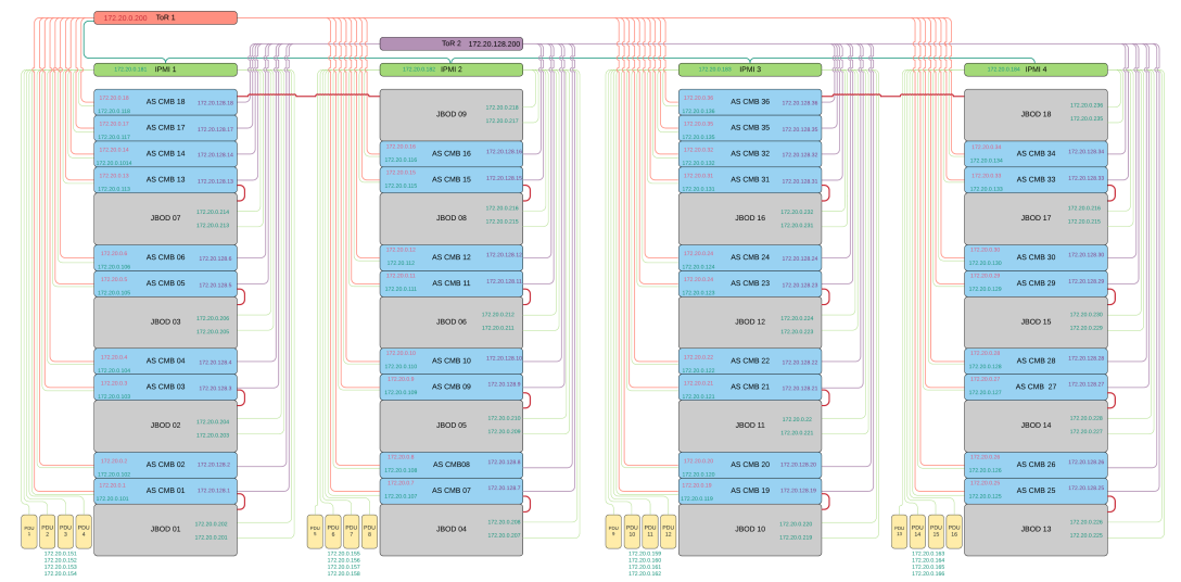
Complete example for a rack, assuming Rack #0 in GEO 1, and assuming 9 chassis / rack:

Node addresses on Private Network 1: 172.21.0.1-36   on VLAN 1000 Node addresses on Private network 2: 172.21.128.1-36 on VLAN 1128 Node IPMI addresses: 172.21.0.101-136   on VLAN 1000    (Private Network 1) JBOD IPMI addresses: 172.21.128.201-236 on VLAN 1128    (Private Network 2)

The reference network cabling for the 2 Public Networks for an X200 deployment would connect to two customer switches (sw-cus-1 and sw-cus-2) for high availability. These customer IP subnets may not overlap with the ActiveScale internal network addresses and would typically use two /24 networks in the 192.168.0.0/16 address block or two /24 networks in the 10.0.0.0/8 address block, as in the example below. Customers may connect both Public Networks to a single switch. Using the ToR switches used by ActiveScale for the public network is possible but discouraged, as it will quickly limit scale-out options.

ActiveScale X200 Racked 6 Twin Plus JBOD and Customer Switches

Depending on the number of nodes in a single column, not all interfaces on the nodes need to be connected to the customer network. The table below lists the number of recommended connected interfaces, and the number of interfaces needed to reach the maximum throughput with large objects. The recommended connected interfaces takes into account that small objects/files benefit from more connections. It is recommended to spread the connections over the 2 customer switches and connect all nodes before using multiple connections on the same node.

Column Nodes	Recommended Connected Customer Interfaces	Throughput Bottleneck
6	12 (all nodes, all interfaces)	7 interfaces
12	16 interfaces, spread over nodes and networks	13 interfaces
18	22 interfaces, spread over nodes and networks	19 interfaces
24	28 interfaces, spread over nodes and networks	25 interfaces
30	32 interfaces, spread over nodes and networks	30 interfaces
36	38 interfaces, spread over nodes and networks	36 interfaces

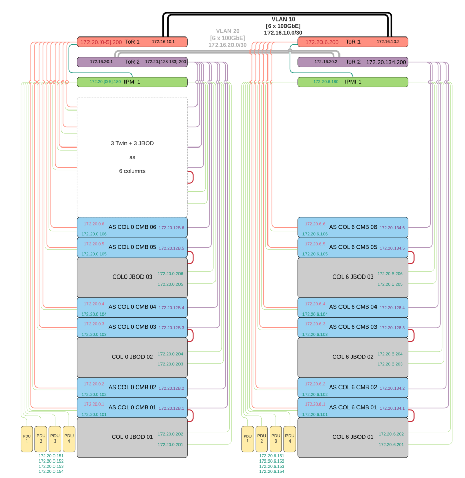
We support 36 nodes per switch (pair). This can be a single 36-node column, 2x 18-node column, etc up to 6x6-node columns. Each column C is configured on separate VLAN-pairs (1000 + C, 1128 + C) and subnets (172.2x.C.0/24 and 172.2x.C+128.0/24).

There is no difference in cabling between the 18 twin + 18 JBOD and 6 times (3 twin + 3 JBOD) setups, but the IP subnets and switch (VLAN) configuration will be different.

For combined systems, traffic within a column is optimized to not send data between scaler and dss over the network. Requests to a column that require access to another column will require a lot more bandwidth in the remote column's private network. From the numbers above, it is expected to be slightly bottlenecked for GETs from a remote system (more with JBODs?). The network bandwidth is 50 Gb/s per node, hardware throughput from disks is about 24 Gb/s per node. A remote GET will cause both the erasure encoded traffic (within the column) and the assembled object (out toward the requesting column) to traverse the same network. Since the erasure encoded blocks will be slightly more bandwidth than the object (so a bit over 2 factor for the total traffic), we are close to the bottleneck for GETs. For PUT the same calculation shows the 50Gb/s bandwidth on the remote cluster will suffice: the throughput per node was ~2.1 GB/s, so close to 12 GB/s for a 2-twin column. Per node that is 2.1 GB/s * 8 = 16.8 Gb/s * 2.3 ~ 40Gb/s, which is within the available bandwidth of 50 Gb/s per node. The impact will be big when a ToR switch should go down. Local requests within a column will be very little affected, but remote requests to another column will show (over) 50% throughput loss.

ActiveScale X200 Racked 6 X 3 Twin Plus JBOD

Scaling out an X100 with X200 is straightforward and only requires connecting the corresponding ToR switches via SFP, which will be limited to the 40GbE speed of the X100 ToR switches. For that, we recommend to NIC-bond the trunk using 2 ports to a combined 80 Gb/s speed. For converged scale out, the base X100 will need to stay connected to the customer network. For full scale out, it is recommended to focus cabling the X200. X100 performance of about 7GB/s =~ 56 Gbit/s can all be handled over the trunk, even in the case of loss of an X200 ToR switch. If an X100 ToR switch is lost, the X100 storage network will become a bottleneck at 60Gb/s.

ActiveScale Racked X100 Plus X200 Scale Out

The figure here is drawn for the first X200 scale out column added to an X100 base rack. After that, the X200 can be scaled out further as before until the ToR switches reach their limit of 36 nodes.

Scaling out X200 beyond an 18 Twin + 18 JBOD setup can be done to up to 3 such clusters by interconnecting the ToR switches. The maximum bandwidth for the uplink between clusters is 6x100 Gb/s + 11x25Gb/s = 875Gb/s when using all remaining ToR ports, which should be enough for the 102 GB/s throughput to scale out to two full 18 Twin clusters. Using only the 100GbE uplinks will already bottleneck the system in case of a switch failure.

ActiveScale X200 Scale Out Network Racked Twin Plus JBOD

Scale out to 3 clusters is still feasible without adding switches and by connecting the ToRs directly.
I would recommend to complete a full mesh with VLANs, as drawn below. Each trunk link uses a single VLAN.

ActiveScale X200 Scaleout 3 Clusters

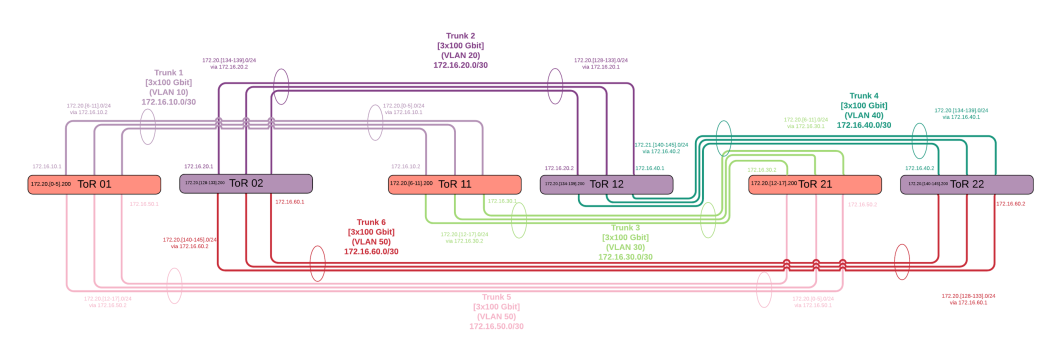
There can be at most six columns known on a pair of ToR switches, so at most 6 /24 networks need to be routed. Routes can be aggregated to require only 2 or 3 routing entries in each switch per trunk (so 4 entries in total) by using /23 and /22 for some entries.
As an example, for ToR 01 and ToR 11, the trunk entries are shown below:

Trunk Routes	ToR 01	ToR 11
non-aggregated	172.20.6.0/24 via 172.16.10.2 172.20.7.0/24 via 172.16.10.2 172.20.8.0/24 via 172.16.10.2 172.20.9.0/24 via 172.16.10.2 172.20.10.0/24 via 172.16.10.2 172.20.11.0/24 via 172.16.10.2 172.20.12.0/24 via 172.16.50.2 172.20.13.0/24 via 172.16.50.2 172.20.14.0/24 via 172.16.50.2 172.20.15.0/24 via 172.16.50.2 172.20.16.0/24 via 172.16.50.2 172.20.17.0/24 via 172.16.50.2	172.20.0.0/24 via 172.16.10.1 172.20.1.0/24 via 172.16.10.1 172.20.2.0/24 via 172.16.10.1 172.20.3.0/24 via 172.16.10.1 172.20.4.0/24 via 172.16.10.1 172.20.5.0/24 via 172.16.10.1 172.20.12.0/24 via 172.16.30.2 172.20.13.0/24 via 172.16.30.2 172.20.14.0/24 via 172.16.30.2 172.20.15.0/24 via 172.16.30.2 172.20.16.0/24 via 172.16.30.2 172.20.17.0/24 via 172.16.30.2
aggregated	172.20.6.0/23 via 172.16.10.2 172.20.8.0/22 via 172.16.10.2 172.20.12.0/22 via 172.16.50.2 172.20.16.0/23 via 172.16.50.2	172.20.0.0/22 via 172.16.10.1 172.20.4.0/23 via 172.16.10.1 172.20.12.0/22 via 172.16.30.2 172.20.16.0/23 via 172.16.30.2

It is possible to extend the above scheme and chain ToRs using 3x100 Gbit NIC-bonded trunk links (or even extend to a ring). The number of routing entries per switch is still very aggregateable, but the bottleneck on the trunks increases, since aggregated traffic of up to 3 clusters may need to travel over one link. Additional use of 25Gbit ports for the trunk can be considered.

However, the recommended network layout for such large deployments is to use a leaf-spine architecture, as shown below:

ActiveScale X200 Scaleout - Beyond Three Clusters

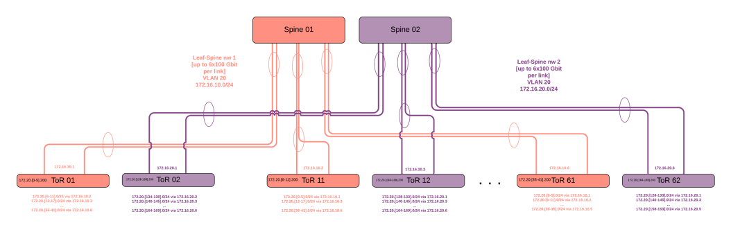
This fabric requires only 2 VLANs, and each ToR switch is connected by a trunk of up to 6x 100Gbit NIC-bonded links to 1 or – recommended – 2 spine switches , which can additionally be augmented using 25 Gbit interfaces. QSPF to 4xSFP+ splitter cables can be used to connect 100GbE ports from the ToR to a 25GbE/100GbE core/spine switch for cost-effectiveness. Customers with 40GbE core switches can use those as well, as the trunk 100GbE ports are 40GbE capable.

Each ToR switches needs up to 6 non-aggregated routes or up to 3 aggreggated routes to reach every cluster in the deployment.